SciML/deSolveDiffEq.jl
Wrappers for calling the R deSolve differential equation solvers from Julia for scientific machine learning (SciML)
deSolveDiffEq.jl
![]()

deSolveDiffEq.jl is a common interface binding for the
R deSolve package of
ordinary differential equation solvers. It uses the
RCall.jl interop in order to
send the differential equation over to R and solve it.
Note that this package isn't for production use and is mostly just for benchmarking
and helping new users migrate models over to Julia.
For more efficient solvers, see the
DifferentialEquations.jl documentation.
Installation
To install deSolveDiffEq.jl, use the following:
Pkg.clone("https://github.com/JuliaDiffEq/deSolveDiffEq.jl")Note that this requires that deSolve is already installed from R and that
RCall.jl is able to appropriately build.
Using deSolveDiffEq.jl
deSolveDiffEq.jl is simply a solver on the DiffEq common interface, so for details see the DifferentialEquations.jl documentation.
The available algorithms are:
deSolveDiffEq.lsoda()
deSolveDiffEq.lsode()
deSolveDiffEq.lsodes()
deSolveDiffEq.lsodar()
deSolveDiffEq.vode()
deSolveDiffEq.daspk()
deSolveDiffEq.euler()
deSolveDiffEq.rk4()
deSolveDiffEq.ode23()
deSolveDiffEq.ode45()
deSolveDiffEq.radau()
deSolveDiffEq.bdf()
deSolveDiffEq.bdf_d()
deSolveDiffEq.adams()
deSolveDiffEq.impAdams()
deSolveDiffEq.impAdams_d()
Example
using deSolveDiffEq

function lorenz(u, p, t)
    du1 = 10.0(u[2]-u[1])
    du2 = u[1]*(28.0-u[3]) - u[2]
    du3 = u[1]*u[2] - (8/3)*u[3]
    [du1, du2, du3]
end
tspan = (0.0, 10.0)
u0 = [1.0, 0.0, 0.0]
prob = ODEProblem(lorenz, u0, tspan)
sol = solve(prob, deSolveDiffEq.lsoda())
Measuring Overhead
deSolveDiffEq.jl has about a 2x-3x overhead over using deSolve in R directly.
To see this, we can time the
main example from the website
library(deSolve)

Lorenz <- function(t, state, parameters) {
  with(as.list(c(state, parameters)), {
    dX <-  a * X + Y * Z
    dY <-  b * (Y - Z)
    dZ <- -X * Y + c * Y - Z
    list(c(dX, dY, dZ))
  })
}

parameters <- c(a = -8/3, b = -10, c = 28)
state      <- c(X = 1, Y = 1, Z = 1)
times      <- seq(0, 100, by = 0.01)

system.time(out <- ode(y = state, times = times, func = Lorenz, parms = parameters))
which outputs
RObject{RealSxp}
   user  system elapsed
   0.33    0.00    0.33
vs the deSolveDiffEq.jl approach:
using deSolveDiffEq, BenchmarkTools

function lorenz(u, p, t)
    du1 = 10.0(u[2]-u[1])
    du2 = u[1]*(28.0-u[3]) - u[2]
    du3 = u[1]*u[2] - (8/3)*u[3]
    [du1, du2, du3]
end
u0 = [1.0; 0.0; 0.0]
tspan = (0.0, 100.0)
prob = ODEProblem(lorenz, u0, tspan)
@btime sol = solve(prob, deSolveDiffEq.lsoda()) # 812.972 ms (2152395 allocations: 67.85 MiB)
Implementation Note
Note that the implementation requires that the function returns a list, so an
R list is generated on the output of each user function call. This means this
is more comparable to the timings of the standard deSolve usage, and not the
C/Fortran function version. We are working to see if that interface can be
directly accessible by Julia functions to check the "expert's version" call
overhead
Benchmarks
The following benchmarks demonstrate a 1000x performance advantage for the
pure-Julia methods over the deSolve ODE solvers across
a range of stiff and non-stiff ODEs*. These were ran with Julia 1.2, MATLAB
2019B, deSolve 1.2.5, and SciPy 1.3.1 after verifying negligible overhead on
interop.
* There is a caveat: this is comparing the "R form" code vs the pure Julia code.
If one directly writes C/Fortran files and compiles that using the
compiled code interface,
the deSolve LSODA matches the performance of LSODA.jl and other pure C/Fortran
calls. Thus this only applied to the standard deSolve usage.
Non-Stiff Problem 1: Lotka-Volterra
f = @ode_def_bare LotkaVolterra begin
    dx = a*x - b*x*y
    dy = -c*y + d*x*y
end a b c d
p = [1.5, 1, 3, 1]
tspan = (0.0, 10.0)
u0 = [1.0, 1.0]
prob = ODEProblem(f, u0, tspan, p)
sol = solve(prob, Vern7(), abstol = 1/10^14, reltol = 1/10^14)
test_sol = TestSolution(sol)

setups = [Dict(:alg=>DP5())
          Dict(:alg=>dopri5())
          Dict(:alg=>Tsit5())
          Dict(:alg=>Vern7())
          Dict(:alg=>MATLABDiffEq.ode45())
          Dict(:alg=>MATLABDiffEq.ode113())
          Dict(:alg=>SciPyDiffEq.RK45())
          Dict(:alg=>SciPyDiffEq.LSODA())
          Dict(:alg=>SciPyDiffEq.odeint())
          Dict(:alg=>deSolveDiffEq.lsoda())
          Dict(:alg=>deSolveDiffEq.ode45())
          Dict(:alg=>CVODE_Adams())]

names = ["Julia: DP5"
         "Hairer: dopri5"
         "Julia: Tsit5"
         "Julia: Vern7"
         "MATLAB: ode45"
         "MATLAB: ode113"
         "SciPy: RK45"
         "SciPy: LSODA"
         "SciPy: odeint"
         "deSolve: lsoda"
         "deSolve: ode45"
         "Sundials: Adams"]

abstols = 1.0 ./ 10.0 .^ (6:13)
reltols = 1.0 ./ 10.0 .^ (3:10)
wp = WorkPrecisionSet(prob, abstols, reltols, setups;
    names = names,
    appxsol = test_sol, dense = false,
    save_everystep = false, numruns = 100, maxiters = 10000000,
    timeseries_errors = false, verbose = false)
plot(wp, title = "Non-stiff 1: Lotka-Volterra")
Non-Stiff Problem 2: Rigid Body
f = @ode_def_bare RigidBodyBench begin
    dy1 = -2*y2*y3
    dy2 = 1.25*y1*y3
    dy3 = -0.5*y1*y2 + 0.25*sin(t)^2
end
prob = ODEProblem(f, [1.0; 0.0; 0.9], (0.0, 100.0))
sol = solve(prob, Vern7(), abstol = 1/10^14, reltol = 1/10^14)
test_sol = TestSolution(sol)

setups = [Dict(:alg=>DP5())
          Dict(:alg=>dopri5())
          Dict(:alg=>Tsit5())
          Dict(:alg=>Vern7())
          Dict(:alg=>MATLABDiffEq.ode45())
          Dict(:alg=>MATLABDiffEq.ode113())
          Dict(:alg=>SciPyDiffEq.RK45())
          Dict(:alg=>SciPyDiffEq.LSODA())
          Dict(:alg=>SciPyDiffEq.odeint())
          Dict(:alg=>deSolveDiffEq.lsoda())
          Dict(:alg=>deSolveDiffEq.ode45())
          Dict(:alg=>CVODE_Adams())]

names = ["Julia: DP5"
         "Hairer: dopri5"
         "Julia: Tsit5"
         "Julia: Vern7"
         "MATLAB: ode45"
         "MATLAB: ode113"
         "SciPy: RK45"
         "SciPy: LSODA"
         "SciPy: odeint"
         "deSolve: lsoda"
         "deSolve: ode45"
         "Sundials: Adams"]

abstols = 1.0 ./ 10.0 .^ (6:13)
reltols = 1.0 ./ 10.0 .^ (3:10)
wp = WorkPrecisionSet(prob, abstols, reltols, setups;
    names = names,
    appxsol = test_sol, dense = false,
    save_everystep = false, numruns = 100, maxiters = 10000000,
    timeseries_errors = false, verbose = false)
plot(wp, title = "Non-stiff 2: Rigid-Body")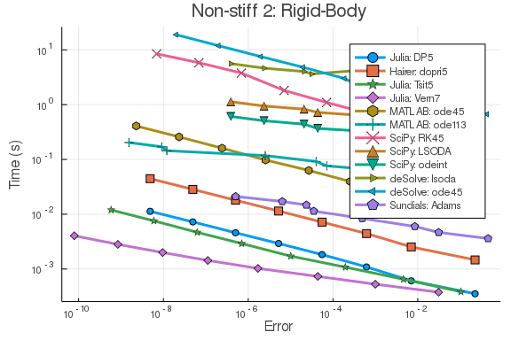
Stiff Problem 1: ROBER
rober = @ode_def begin
    dy₁ = -k₁*y₁+k₃*y₂*y₃
    dy₂ = k₁*y₁-k₂*y₂^2-k₃*y₂*y₃
    dy₃ = k₂*y₂^2
end k₁ k₂ k₃
prob = ODEProblem(rober, [1.0, 0.0, 0.0], (0.0, 1e5), [0.04, 3e7, 1e4])
sol = solve(prob, CVODE_BDF(), abstol = 1/10^14, reltol = 1/10^14)
test_sol = TestSolution(sol)

abstols = 1.0 ./ 10.0 .^ (7:8)
reltols = 1.0 ./ 10.0 .^ (3:4);

setups = [Dict(:alg=>Rosenbrock23())
          Dict(:alg=>TRBDF2())
          Dict(:alg=>RadauIIA5())
          Dict(:alg=>rodas())
          Dict(:alg=>radau())
          Dict(:alg=>MATLABDiffEq.ode23s())
          Dict(:alg=>MATLABDiffEq.ode15s())
          Dict(:alg=>SciPyDiffEq.LSODA())
          Dict(:alg=>SciPyDiffEq.BDF())
          Dict(:alg=>SciPyDiffEq.odeint())
          Dict(:alg=>deSolveDiffEq.lsoda())
          Dict(:alg=>CVODE_BDF())]

names = ["Julia: Rosenbrock23"
         "Julia: TRBDF2"
         "Julia: radau"
         "Hairer: rodas"
         "Hairer: radau"
         "MATLAB: ode23s"
         "MATLAB: ode15s"
         "SciPy: LSODA"
         "SciPy: BDF"
         "SciPy: odeint"
         "deSolve: lsoda"
         "Sundials: CVODE"]

wp = WorkPrecisionSet(prob, abstols, reltols, setups;
    names = names, print_names = true,
    dense = false, verbose = false,
    save_everystep = false, appxsol = test_sol,
    maxiters = Int(1e5))
plot(wp, title = "Stiff 1: ROBER", legend = :topleft)
Stiff Problem 2: HIRES
f = @ode_def Hires begin
    dy1 = -1.71*y1 + 0.43*y2 + 8.32*y3 + 0.0007
    dy2 = 1.71*y1 - 8.75*y2
    dy3 = -10.03*y3 + 0.43*y4 + 0.035*y5
    dy4 = 8.32*y2 + 1.71*y3 - 1.12*y4
    dy5 = -1.745*y5 + 0.43*y6 + 0.43*y7
    dy6 = -280.0*y6*y8 + 0.69*y4 + 1.71*y5 -
          0.43*y6 + 0.69*y7
    dy7 = 280.0*y6*y8 - 1.81*y7
    dy8 = -280.0*y6*y8 + 1.81*y7
end

u0 = zeros(8)
u0[1] = 1
u0[8] = 0.0057
prob = ODEProblem(f, u0, (0.0, 321.8122))

sol = solve(prob, Rodas5(), abstol = 1/10^14, reltol = 1/10^14)
test_sol = TestSolution(sol)

abstols = 1.0 ./ 10.0 .^ (5:8)
reltols = 1.0 ./ 10.0 .^ (1:4);

setups = [Dict(:alg=>Rosenbrock23())
          Dict(:alg=>TRBDF2())
          Dict(:alg=>RadauIIA5())
          Dict(:alg=>rodas())
          Dict(:alg=>radau())
          Dict(:alg=>MATLABDiffEq.ode23s())
          Dict(:alg=>MATLABDiffEq.ode15s())
          Dict(:alg=>SciPyDiffEq.LSODA())
          Dict(:alg=>SciPyDiffEq.BDF())
          Dict(:alg=>SciPyDiffEq.odeint())
          Dict(:alg=>deSolveDiffEq.lsoda())
          Dict(:alg=>CVODE_BDF())]

names = ["Julia: Rosenbrock23"
         "Julia: TRBDF2"
         "Julia: radau"
         "Hairer: rodas"
         "Hairer: radau"
         "MATLAB: ode23s"
         "MATLAB: ode15s"
         "SciPy: LSODA"
         "SciPy: BDF"
         "SciPy: odeint"
         "deSolve: lsoda"
         "Sundials: CVODE"]

wp = WorkPrecisionSet(prob, abstols, reltols, setups;
    names = names, print_names = true,
    save_everystep = false, appxsol = test_sol,
    maxiters = Int(1e5), numruns = 100)
plot(wp, title = "Stiff 2: Hires", legend = :topleft)